Table of Contents
Introduction
In 1996 Chuck Doswell, Harold Brooks, and Robert Maddox published an important paper outlining an “ingredients-based methodology” for flash flood forecasting. They pointed out that rainfall accumulation depends on its intensity times its duration. The paper emphasized the role of vertical lift, moisture content, and the efficiency with which water vapor is converted to rainfall (precipitation efficiency) as the three primary ingredients of intensity, and storm size, motion, and orientation as key to determining rainfall duration.
About a decade later, additional research by Schumacher and Johnson showed that major flash flood-producing systems tend to organize in two ways: training line/adjoining stratiform (TL/AS) and back-building (BB). TL/AS systems consist of a line of storms that pass the same location in succession, like a train traveling down a track. A broader region of more moderate, stratiform rainfall tends to be situated north of the line of storms. Back-building systems are backward-propagating: new storms form to the rear of existing cells. Both training and back-building prolong the duration of rainfall over the same area, accumulating rainfall and making flash flooding more likely.
The Meteorological Process Mapper
I’m in the latter stages of developing a new tool for analyzing weather balloon soundings that I call the Meteorological Process Mapper (MPM). While traditional sounding analysis involves threshold-based parameters and indices to predict severe and hazardous weather, MPM instead takes the approach of exploring the “anatomy” of the atmosphere, using a hierarchical structure of parameters that are weighted and combined to form processes that represent important interactions.
Essentially, MPM performs a decomposition of the atmosphere, separating a convective environment into interacting dynamical, thermodynamical, and microphysical subsystems in order to reveal how the larger atmospheric state organizes its behavior. Key lower-order processes are combined and weighted to form higher-order processes. (I recommend reading my process-based framework for some insight into the underpinnings of MPM.) The result is a system that can diagnose how the atmosphere constructs storms and precipitation systems to produce hazards, such as severe wind, hail, tornadoes, and floods.
Because Doswell et al. laid out such a clear template for flash floods – it’s not much of a leap to transform their “ingredients” into “processes” – investigating a dataset of major flash floods seemed like a logical starting point to test MPM. Starting here also brings me back to my academic roots, as both my Master’s and Ph.D. work investigated flash floods in the northeast U.S.
But which floods to include? I wanted to keep the dataset small. I found a Wikipedia list of major flash flood events and extracted those from the U.S. (along with one in Canada). I added one from my earlier work and another recent event to round out the sample size at 29. I downloaded the nearest sounding to each flood from the morning and evening, ran the data through MPM, and created some graphics to visualize the results.
Flash Flood Analysis
As MPM is still in development and subject to continued testing, this analysis is limited to a small set of seven variables:
Convective Available Potential Energy (CAPE) – the buoyant energy available for parcels to continue to rise freely, once they become more buoyant than their surrounding environment. It’s expressed as an index from 0 to 1, and any values that exceed a specified threshold are equal to 1.
Precipitable water (PWAT) index – the total water vapor in the air column. This, too, is an index, ranging from 0 to 1, and capped at a threshold.
Precipitation efficiency – a measure of the conversion of water vapor to liquid water. In MPM, precipitation efficiency is a composite of several sub-processes.
Updraft budget – represents the potential for vertical lift. To find the updraft budget, CAPE is scaled to provide an estimate of upward vertical motion, and then modified based on a few factors that can slow this rising motion. In other words, CAPE is the raw potential for rising motion, while the updraft budget attempts to corral that potential into a more reasonable estimate based on processes that may impede it given the conditions in the sounding.
Training potential – potential of storm cells to repeatedly pass over the same area in succession.
Stationarity factor – indicates how likely storm cells are to remain quasi-stationary.
Back-building potential – potential for storm cells to continually reform at the rear of existing cells, producing long-duration, quasi-stationary rainfall.
Overall Results
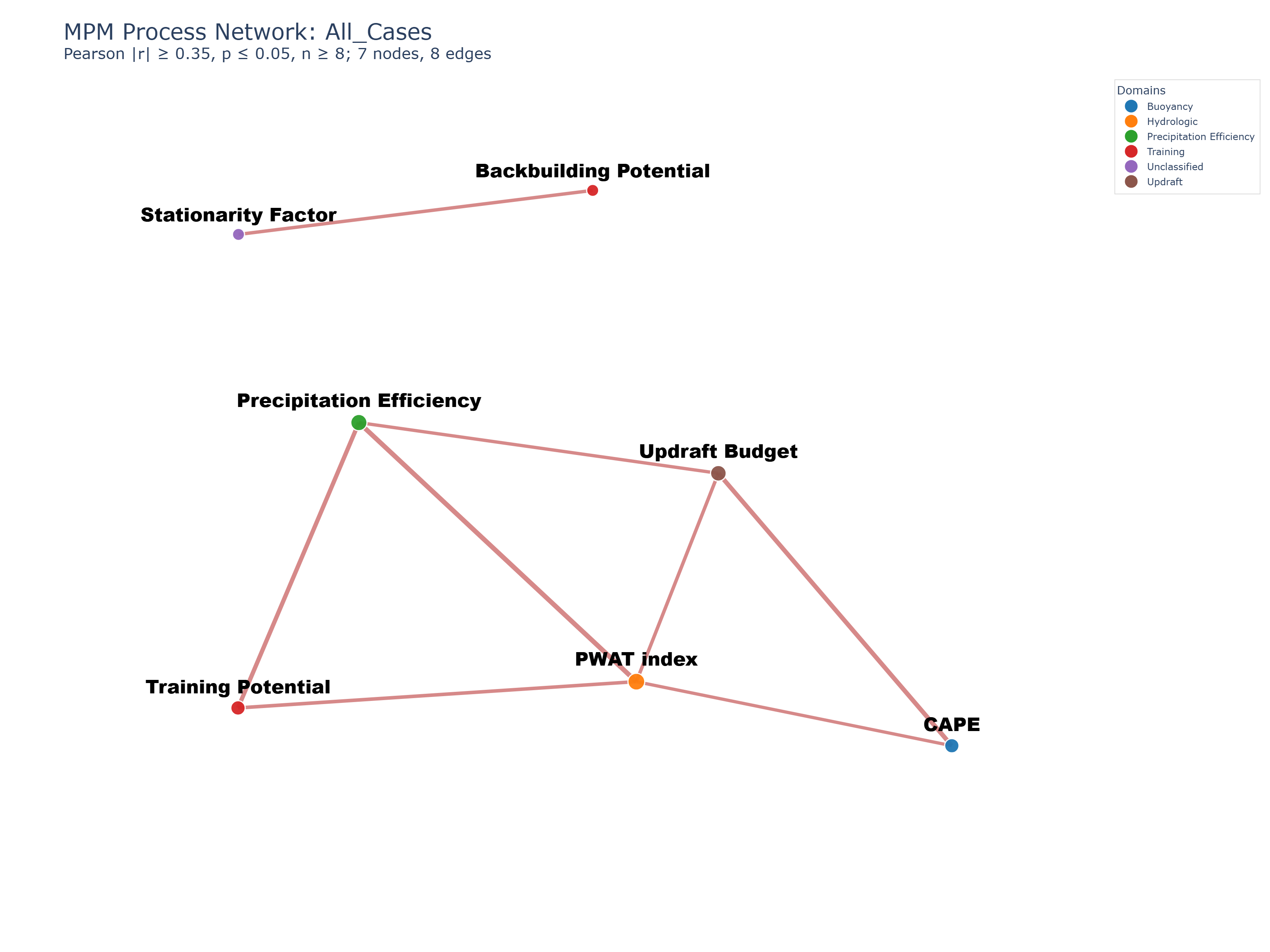
Here is the network map of these seven variables across both morning and evening, as observed in the 29 cases in my dataset:

Each process is indicated by a node, which is color-coded by the type of process. The size of the node indicates its importance in the network. A red connector between nodes indicates a direct relationship between the two connected variables, where both variables increase or decrease concurrently. A blue connector indicates an inverse relationship, where one variable increases as the other decreases. The thickness of the connecting lines is directly proportional to the strength of the correlation between the connected parameters. The distance between points is inconsistent: don’t try to judge the strength of connections by how closely spaced the points are!
In this network, all relationships are direct. This suggests that the major flash flood environments for these events are characterized less by tradeoffs between competing processes and more by cooperative amplification: a moister environment is more efficient; a more efficient environment supports rainfall persistence through training, stationarity, and backbuilding; and buoyancy fuels the vertical transport engine that supports it all. This is the essence of the Doswell et al. framework.
Perhaps more relevantly, the relationships appear to validate MPM as capable of uncovering and expressing of that framework. The largest node is PWAT index, with a degree of 4. Thus, the total moisture content in the vertical column has the most organizational influence within the network. This also suggests that the availability of moisture may constrain the extent to which other processes in the system can be realized. Fortunately for the raindrops, there is a lot of moisture in these environments!
Both Precipitation Efficiency and Updraft Budget have a degree of 3, their central presence in agreement with Doswell et al.’s ingredients-based framework. Notably, the Updraft Budget, which refines and modifies CAPE, is more central to the network than CAPE alone. The positions of Updraft Budget and CAPE at one end of the network rather than in the center suggest that buoyancy helps to establish convection, but rainfall intensity may emerge more from how moisture, efficiency, and storm organization interact afterward, as we will see when we look at the network map for the evening soundings.
Along with CAPE, training potential bookends the inner triangle of lift, moisture, and efficiency. Even though Training Potential is conceptually more aligned with Back-building and Stationarity factor, it is statistically more closely connected to intensity production for this set of cases. The Training Potential and Stationarity Factor connections are also notable because they attach more strongly to the hydrologic side of the network than to the buoyancy side, while Back-building sits more directly in the center. Notably, the set of [PWAT index, Precipitation Efficiency, and Training Potential] appears to be more closely related than the set of [PWAT index, Updraft Budget, and CAPE], as you can see in the correlation matrix below.
The rows and columns for PWAT, Precipitation Efficiency, and Updraft Budget are highlighted in yellow, and statistically significant correlations are shaded in red, with darker shading corresponding to greater statistical significance. The table makes it clear that PWAT is the central axis around which the other variables orbit, and the networked nature of the map is apparent from the many statistically significant correlations across the table.

The larger sample size of the combined dataset makes clear the relationships that govern the intensity and duration of heavy rainfall producing flash floods, and these relationships depict the theoretical framework of Doswell et al. amazingly well. When this dataset is broken down by time of day, different structures appear, as some relationships become more significant, while others are dissolved.
The rest of this post is password-protected.
Conclusion
My choice to examine flash floods as a first step in validating MPM proved to be prescient. I anticipated that the simple formulation of flash flooding in the literature would translate well to MPM architecture, and this was borne out in the results. MPM works best in analyzing smaller datasets that are well-constrained; this dataset was constrained by the magnitude of flooding and its impact. Perhaps because a wide variety of scenarios were represented, the network maps agreed remarkably well with the theoretical framework governing flash floods.
The relationships that MPM uncovers are quite sensitive to the composition of cases examined. Had I instead constructed a larger dataset, parsed the network maps by region, and considered only events occurring during the afternoon, different regions would have displayed a unique process network. A Desert Southwest flood is very different from one in the Northeast, and MPM is capable of showing why.
This post uncovered a rich trove of insights from a small dataset with only seven parameters. MPM’s scope is much larger: it defines about 40 processes and many, many more terms and variables that contribute to those processes. Imagine a network map consisting of 15, 25, or more nodes and the complex web of relationships that they would connect…and how much more insight that level of detail can provide. This is where MPM is headed.
What’s next for MPM? I plan to continue refining the code and testing it with different datasets. I’d especially like to see how it diagnoses environments that produced large tornadoes and giant hail. Eventually, hopefully sooner than later, I’ll release the code publicly so others can experiment with it. I’m excited to see where it leads. But for now, it’s back to work…
References
Doswell , C. A., H. E. Brooks, and R. A. Maddox, 1996: Flash Flood Forecasting: An Ingredients-Based Methodology. Wea. Forecasting, 11, 560–581, https://doi.org/10.1175/1520-0434(1996)011<0560:FFFAIB>2.0.CO;2.
Schumacher, R. S., and R. H. Johnson, 2006: Characteristics of U.S. Extreme Rain Events during 1999–2003. Wea. Forecasting, 21, 69–85, https://doi.org/10.1175/WAF900.1.
Want to receive future posts in your inbox? Be sure to subscribe to this blog using the “Newsletter” link at upper right. This work is made possible by those who believe in it. Thank you for considering a gift to help ensure its continued momentum.
Author’s Note: This summary is freely available for educational use. Please cite “Jessup, S. (2026). A Process Analysis of Major Flash Floods” in scholarly work.
