Table of Contents
Setting Up the Experiment
As I was teaching my environmental air quality course in 2022, a local business was under scrutiny for emissions of a substance – carbon black – that was soiling people’s clothes, pets, cars, and homes. I used some available funds to purchase air quality sensors that could detect aerosol particles (particulate matter), and we did some sampling around a neighborhood that was affected by the pollution. We didn’t find much because most of the pollution was occurring at night, but the experience sparked my interest in studying aerosols.
More recently, I’ve purchased another set of handheld sensors that can be calibrated and that detect additional gases (carbon dioxide, CO2, and formaldehyde, HCHO). In this post, I’m going to discuss a set of measurements I made with these sensors on December 12, 2025 and how these observations may provide evidence for my recent discovery: the Subcritical Aerosol-Moisture Feedback.

It measures temperature, relative humidity, particulate matter, CO2, and HCHO.
On December 12, I unpacked the sensors only to discover that one of the three was nearly out of charge. I set up the two functional sensors on an 8-foot ladder on my back deck. I placed one sensor on the bottom rung and the other sensor on top of the ladder. After more sensors arrive, I will be able to place one on each rung and have a detailed picture of vertical exchange processes in this near-surface layer.

The sensors have limited battery power: they can run for about seven hours on a full charge. They have to be handled carefully, as they can’t be exposed for long to below-freezing temperatures, relative humidity greater than 90%, or long durations of high aerosol exposure. On December 12, these conditions weren’t a concern to start with, as it was plenty warm and the air wasn’t too humid. I expected to keep the sensors recording for a few hours, and bring them inside in the evening when the humidity had climbed too high. I only needed the first 75 minutes to find something pretty exciting.
The Objective of the Experiment
I wanted to capture the evening transition because it’s an important interval when the temperature falls, relative humidity increases, and aerosols can grow. During the evening transition, turbulence weakens and smaller-scale interactions take over. I wasn’t sure what I was going to find, but I knew there would be something interesting. I suspected that the differences between the two sensors might convey something about the microphysical interactions between the aerosol particles and humidity that form the basis of the Subcritical Aerosol-Moisture Feedback, which will be discussed later. My main interest was in capturing how the thermodynamic state (temperature and humidity) of the near-surface air evolved from late afternoon into the evening and how aerosols respond.
I’ve been evaluating the hypothesis that a climate regime shift occurred around November 20, 2025. My first suspicion that something fundamental had changed came from my observations of clouds beginning on that date. I had been planning to make some measurements with my particulate matter sensors during winter break, and the suspected climate regime shift provided additional motivation. Such a regime shift involves reorganization at all scales of the atmosphere, so with this first observation day of my winter break, I was hoping to find something that perhaps hadn’t been seen before…something that could help explain how the new climate regime organizes differently than the patterns we are used to.
I completed my calibration and setup, and the sensors were ready to roll shortly before 4:00 pm EST (16:00). In my post-processing, I trimmed the first few minutes of data recorded while the sensors equilibrated with their environment. The record begins at 4:05 pm.
Temperature and Relative Humidity Evolution
The graph below shows the air temperature (T; °F) for the two sensors. The warmer, red (solid) sensor was at the bottom of the ladder, and the cooler, purple (dashed) sensor was at the top. For each sensor, I emphasize the raw data (bold line), with a thinner line representing the 10-minute mean (smooth, thinner line).

At the top of the ladder (purple), the temperature declines steadily. While this higher air shows little variability around its declining temperature trend, the air temperature close to the ground (red) oscillates with greater variability from the beginning until it begins to cool at 4:30 pm (16:30 on the graph). Once the air at this bottom sensor begins to cool, it does so more rapidly than in the air above, until the last few minutes, when both curves flatten and their variability increases.
These rapid initial temperature fluctuations are associated with turbulence. Even though the wind speed was minimal, variability in temperature due to solar heating produces thermal turbulence during the day as whirls of air, known as turbulent eddies, are produced by small scale temperature contrasts. If you look at a blacktop surface on a hot, sunny day, the rippling waves of air motion you see just above the asphalt are created by thermal turbulence.

Source: https://blacktoppassages.com/2014/09/09/563/
The air temperature graph above (Figure 3) suggests that this thermal turbulence was confined low to the ground because the sensor at the top of the ladder (purple) did not exhibit the same variability as the lower sensor (red). The reduction in variability of the red line as the temperature begins to decline around 4:30 pm suggests a reduction in thermal turbulence as the sun descends.
This weakening of thermal turbulence occurred well before sunset. The sky was clear, but the top of the ladder may have been overtaken by shadow around 4:30. The bottom sensor, where the air was most turbulent, was in shadow for the duration of the record.
The graph below shows the dewpoint temperature (Td; °F) for the same time period, showing only the raw data, but with the same colors as before. The dewpoint temperature is a direct indicator of humidity: when the dewpoint temperature is higher, the air contains more water vapor.

of the ladder from 4:05 pm to 5:12 pm, December 12, 2025 in Columbus, GA.
Notice the numbers on the vertical axis: the difference in Td between the top and bottom of the ladder was less than 2°F, while the difference in T on Figure 3 reached as high as 10°F. While the temperature field has a large vertical gradient, these dewpoint measurements show that the humidity field is more vertically uniform. However, Td remains noisier throughout the graph, so this moisture field tends to vary more through time around its upward trend.
Also notice Td is higher at the bottom of the ladder (the red line is now on top), and Td is lower above (purple line). Surface evaporation is the primary source of moisture to the near-surface layer; the moisture is greatest at the bottom.
Throughout the early portion of this data record, Td acts in a general inverse manner: when it increases at the top, it decreases at the bottom, and vice versa. Beginning at 16:48, the lines come closer together: the vertical moisture gradient decreases. At about 17:05, the lines separate again but respond roughly in phase with each other to the end of the period. We will see soon that aerosol concentrations were locked into the same oscillations from 17:05. This tightly in-phase behavior between aerosols and moisture is evidence that suggests the Subcritical Aerosol-Moisture Feedback is strongly active.
I find it surprising that the dewpoint was climbing steadily as the sun sank. Usually, changes in Td operate more in tandem with T, declining during the evening. Winds were weak, so there was little transport of moisture from elsewhere. In my last blog post, I discussed a case where changes in Td appeared to result from a vertical redistribution of moisture from above. It’s possible that the same kind of mechanism is operating here, but we’ll save this question for a future post.
Now let’s consider how the relative humidity (RH) changes through time. RH is proportional to the difference between T and Td. When T is warmer for the same amount of moisture (constant Td), RH is lower and the air is less saturated. In the RH graph below, the warmer air near the ground (red) is farther from saturation (lower RH), and the cooler air above (purple) is closer to saturation (higher RH). Over time, as the air cools, RH increases for both sensors.

Both T and Td were initially more variable at the top of the ladder (red). Because it is proportional to their difference, RH shares that variability here. After the initial turbulence dissipates (around 16:30), RH increases smoothly. After this time, the variations in Td that we saw in Figure 5 produce only weak variations in RH because T oscillates in similar fashion.
At the bottom of the ladder (purple), the variability is much lower from the beginning. The smoothed RH curve generally increases from one time step to the next throughout the duration of the curve (we call this “monotonic“), with the rate of increase only slightly increasing at first but becoming steeper beginning around 16:20.
Meanwhile, RH at the top of the ladder (red) begins to increase at a faster rate once the variability is reduced around 16:30, and the rate of increase slows slightly beginning around 16:50. RH typically increases through the evening. Here, the layer moisture is becoming increasingly homogenized as the lines converge.
Aerosol Growth
PM2.5 Data
As RH increases, the air comes closer to saturation. As the air saturates, aerosol particles can retain more water over time, and as residence time increases, the aerosols grow. Generally, we quantify aerosols based on their size, dividing them into two groups: PM2.5 and PM10, where the numbers represent the threshold diameter of the aerosol in microns (or micrometers). PM2.5 are small particles, and PM10 are larger particles. Rather than counting the number of particles for each size threshold, the PM variables quantify them by their total mass, in micrograms per meter cubed.
The graph below shows the time series for PM2.5 over the time window we have been examining. Unlike the T and RH data, the PM2.5 data maintain a consistent, nontrivial amount of variability throughout – even after the rates of change in T and RH become steady. In general, the range of variability is similar for both sensors, but the magnitude of PM2.5 separates about halfway through, with a higher mass developing at the bottom of the ladder.

from 4:05 pm to 5:12 pm, December 12, 2025 in Columbus, GA.
We can infer that the increase in mass of these small aerosols is dominated by particle production, rather than the growth of existing particles, because the number of particles is increasing in the same manner, in terms of the rate of change, the variability, and the separation between layers. Notice the strong similarity between the graph of particle count below and PM2.5 above.

from 4:05 pm to 5:12 pm, December 12, 2025 in Columbus, GA.
How Aerosols Moisten
Individual aerosol particles don’t go from dry to wet in a continuous, linear fashion; they jump from a drier state to a wetter state once a specific RH threshold is reached. This jump is known as deliquescence, and the RH threshold at which the jump occurs depends on the chemical composition of the aerosol. When the air dries, aerosols experience the opposite (downward) jump, which is known as efflorescence.
When atmospheric conditions are sustained near a deliquescence threshold, this might have the effect of buffering the thermodynamic state of the air, holding T and RH steady even as the aerosol concentration or solar radiation changes via the Subcritical Aerosol-Moisture Feedback. I observed a similar buffering effect during the the April 8, 2024 solar eclipse and reported on it in a peer-reviewed journal article.

Source: Veith et al. 2021, Molecules. (CC BY) license.
The figure above illustrates the deliquescence curve for the simple sugar molecule fructose. The plot is computed for a constant temperature of 298.15 Kelvins (~77 °F) and shows how the water sorption (w_water on the y-axis) suddenly increases when the RH reaches 61.5% (the deliquescence relative humidity, or DRH). In the case of fructose, the substance remains bone dry prior to wetting and forms a crystal when wetted.
Many aerosols in the atmosphere consist of mixed composition rather than a single chemical compound, and they are gradually wetted, even before deliquescence. The rate of wetting increases as the RH approaches the DRH. At first glance, the steepening of the PM2.5 curves in Figure 7 above may suggest that a sub-population of aerosols may be approaching its deliquescence threshold.
However, in this case, the RH is approaching 50%, which doesn’t correspond to the DRH of a predominant aerosol type that would be expected in this environment. The aerosols are growing, but they are remaining in their drier state rather than jumping to a wetted one. Since deliquescence isn’t driving the feedback, the mechanism is likely more subtle.
Growth of Coupling
In this case, the growth is identical across sizes. Figure 10 below compares PM2.5 (top graph) and PM10 (bottom graph) at the top of the ladder. Although it’s not shown, this shared behavior across size also occurs at the bottom of the ladder. Aerosols of all sizes are growing at a uniform rate, rather than a trend for small particles to become larger ones.

While this shared behavior across size is maintained independently at both the top and the bottom of the ladder, it differs when the two levels are compared with each other. As we saw earlier when we compared PM2.5 for the bottom and top of the ladder, the magnitude of PM2.5 separates halfway through the time series. That graph is shown again below. Before reading the discussion below, I invite you to study this graph. How would you segment it into stages based upon the shared PM2.5 activity between the top and bottom layers? Where do the two sensors change randomly, where do they change in the opposite manner, and where do they change in the same manner?
Before 16:40, the PM2.5 values at the top and bottom of the ladder occupy a similar range, but the behavior is somewhat erratic. The bottom sensor displays a higher frequency signal, while aerosols at the top sensor change more slowly. The early tendency toward randomness, or “stochasticity“, becomes more ordered, especially once the top and bottom stratify: PM2.5 briefly becomes phase-locked (or in phase) across levels just before 16:40. Then, the top and bottom mirror each other beginning shortly after 16:40, varying inversely, and finally become largely synchronized, changing more or less in unison from around 17:00.
Overall, the vertical coupling within the system increases substantially from the beginning of the time period to the end. We saw earlier that RH exhibits identical oscillations for the last 10 minutes of the record. We are witnessing a system that transitions from loosely connected to tightly coupled across variables through the depth of the layer.
The PM2.5 data are shown again below, with shaded overlays to display these phase shifts.

annotated with phase relationships.
Regime Shift
The graph below illustrates the differences between the top and bottom of the ladder in our three key variables: T, RH, and PM2.5. This graph shows that the initial separation around 16:40 occurs in a sequence: RH peaks and then begins to decrease around 16:25, T reaches a minimum and begins to rise at 16:30, while the PM2.5 concentration shifts to a lower center about ten minutes later, as shown by the drop in the thin line (the rolling mean).

and PM2.5 (bottom).
The air temperature difference (top graph), exhibits a relatively smooth logarithmic rise, asymptotically approaching a straight line at a value of about -1.5 °F (cooler at the top) by the end of the period. The RH layer difference (middle graph) decreases nearly linearly at first, but its slope flattens with time. The smoothed (10-minute) mean for the PM2.5 layer difference (bottom graph) decreases in roughly stepwise fashion, with the mass of small aerosols abruptly becoming more concentrated near the ground, where the air is cooling more rapidly. Through this transition, the variability in PM2.5 increases.
This separation of PM2.5 between the top and bottom of the ladder suggests a settling of aerosols, providing a hint as to what happened around 16:40. This transition likely marks a regime shift, and the aerosol field adjusts minutes after the temperature and RH curves shift course. I argued earlier that this is around the time that turbulence breaks down, and with it the coupling between kinematic (motion) and thermodynamic (temperature and humidity) processes near the surface becomes greatly reduced. The thermodynamic environment becomes less conditioned by convective motions of the air and more regulated by smaller-scale interactions, in particular aerosol-moisture feedbacks. This allows coupling to emerge between the top and bottom of the ladder.
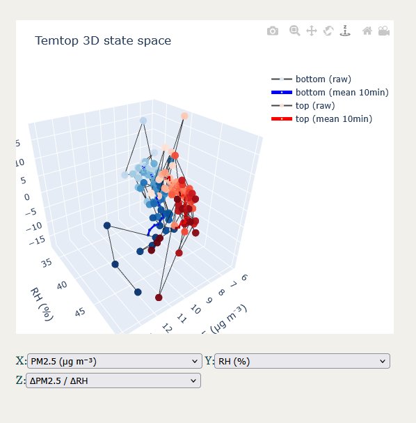
Play With the Data!
When I really want to understand what is going on, I find it helpful to play with the data, especially on 3D plots. Seeing the data in this multidimensional space brings it alive, showing connections between variables. I’ve made a 3D plot available for you to manipulate below. You can change the variable on any axis using the dropdowns below the plot, and you can turn the raw value traces and the mean traces on and off by clicking on their symbols in the legend at upper right. If you are on a desktop, you can click and drag to rotate the view, and you can scroll the mouse wheel to zoom. Mousing over a data point shows their its values. On a mobile or tablet, you can use your finger.
I recommend keeping PM2.5 on the x-axis, RH on the y-axis, and changing the variable on the z-axis. I am intentionally keeping the parameter space small by including only aerosol, temperature, and moisture data. Have fun!
The Subcritical Aerosol-Moisture Feedback
The Subcritical Aerosol-Moisture Feedback (SAMF) involves three interacting constituents: aerosols, water, and photons of light. Aerosols and water vapor form a coupled reservoir, while photons represent the radiative energy field that interfaces with that reservoir. Photons are more directly connected to aerosols because an aerosol’s scattering, absorption, and emission of infrared energy depends on its size and water content, especially once it develops a thin film of water.
These constituents are linked through three coupled processes: aerosol growth via hygroscopic water uptake, radiative interaction between aerosols and photons, and microphysical enthalpy exchange between aerosol-associated water and the surrounding air. Enthalpy is a convenient way to consider the energy of exchanges between a “system” and its surroundings. The change in enthalpy for a process at constant pressure is exactly equal to the heat that flows between the system and the surroundings for that process. The physical and process interactions of SAMF are summarized in Figure 14 below.

of the Subcritical Aerosol-Moisture Feedback.
In this context, enthalpy refers specifically to the thermal energy content associated with the phase state of water, including its internal energy and the work it does on its surrounding environment, that latter of which is associated with volume and pressure. As water is taken up or released by aerosols, enthalpy is exchanged locally between the particle and its environment, influencing the temperature and moisture fields that characterize the thermodynamic state of the layer of air in which the aerosol resides. Through the coupling of aerosol growth with the surrounding temperature and moisture, this growth mediates how moisture and radiation interact under constrained conditions, forming the basis of SAMF.
Hydration and dehydration form the core of the microphysical enthalpy exchange. During water uptake, energy is released at the particle scale into both the particle and its surrounding air; during drying, energy is absorbed from the surrounding environment. This exchange is “microphysical” because it occurs at the scale of particle water films and solution layers, and it is “exchange” because energy is transferred between the water substance, the aerosol, and the local air as the equilibrium partitioning of water adjusts between phases.
In a field of growing aerosols, spatial variations in humidity locally enhance or suppress hygroscopic growth, leading to corresponding heterogeneity in aerosol optical properties. As water films accumulate on aerosol surfaces, particle size and effective emissivity increase, enhancing visible and near-infrared scattering while also increasing longwave absorption and emission by the aerosol field. Increased effective longwave absorptivity and emissivity of the growing aerosol field cause a larger fraction of upwelling infrared radiation to be absorbed and re-emitted locally instead of escaping directly upward.
The combined effect of this hydration and its radiative response is to reduce vertical radiative contrasts by increasing radiative coupling within the layer, rather than by reversing net cooling. This coupling increases the radiative residence time of energy within the layer, slowing the rate of thermal adjustment. As hygroscopic growth becomes sufficiently widespread for absorption and emission to act efficiently, vertical radiative gradients are damped, decreasing the scale of energy propagation kinematically by reducing the influence of buoyant forcing and by further suppressing turbulence.
This enhanced radiative coupling strengthens the phase relationship between moisture and aerosols and their influence on their surroundings. SAMF coupling behavior between moisture and aerosols is illustrated by the in-phase and inverse relationships in PM2.5 between the top and bottom of the ladder in the second half of Figure 12 above, which is shown again below. The coordinated aerosol activity across the layer is enabled by SAMF.
annotated with phase relationships.
Across a population of aerosols, these changes act primarily to dampen thermal and moisture gradients rather than to alter net fluxes. By reducing vertical radiative contrasts and suppressing turbulent exchange, the system loses degrees of freedom for rapid adjustment and instead evolves along an increasingly constrained, slowly varying trajectory. In this sense, the coupled aerosol-moisture field tends to hold the system in a dynamically stabilized state, even as cooling and moistening continue. This gradient-damping, constraint-driven behavior is the essence of the Subcritical Aerosol-Moisture Feedback.
The image below illustrates the Subcritical Aerosol-Moisture Feedback as a chain of causality. The arrows around the outside ring are two-way, except for the first arrow from radiative forcing to RH, indicating that both moistening and drying, growth and decay, or warming and cooling can adjust the system in opposite directions.

In the case we’re examining, a transition from turbulent oscillations to persistent cooling in the air temperature at the bottom of the ladder initiates the intensification of SAMF coupling. As the bottom begins to cool much faster than the top, the temperature difference equilibrates rapidly at first, and then more and more slowly. Mathematically, the temperature difference evolves logarithmically as radiative gradients are damped, while the aerosol field transitions to a faster accumulation regime as residence time increases.

and PM2.5 (bottom).
As turbulence collapses, aerosols become more stratified and spatially heterogeneous, reflecting their sensitivity to local moisture availability and microphysical opportunity. At the same time, temperature and humidity fluctuations are increasingly suppressed because the coupled aerosol-moisture feedback acts primarily to dampen radiative and buoyant gradients. Variability is thus redistributed from the thermodynamic fields into the aerosol field, a defining signature of self-organization under constraint.
This case illustrates how decreases radiative forcing imposes environmental constraints that strengthen the coupling between humidity and aerosols. In future case studies, we will explore other ways the system can evolve.
Want to receive future posts related to this study in your inbox? Be sure to subscribe to this blog using the “Newsletter” link at upper right.
This work is made possible by those who believe in it. Thank you for considering a gift to help ensure its continued momentum.
Author’s Note: This summary is freely available for educational use. Please cite “Jessup, S. (2025). Subcritical Aerosol-Moisture Feedback (SAMF) Case Study: Self-Organization During Evening Transition” in scholarly work.